When estimating machine learning models, the problem of class imbalance often occurs. This means that the target variable is not equally distributed, but unevenly distributed. Usually the positive class is very small, while the negative class is very large, assuming a binary target class.
So what is the problem?
Let us assume the distribution of the binary target variable looks like this:
- 95% negative class
- 5% positive class
To reduce the level of abstraction, we will explain the imbalance problem with an example. Let us assume we want to estimate the purchase of a product: 95% of the customers in my data set did not buy, while only 5% bought. Thus, the positive class (label = 1) is “purchase” and the negative class (label = 0) is “no purchase”. We estimate a model, for example a random forest. The following fictitious confusion matrix serves as illustration:
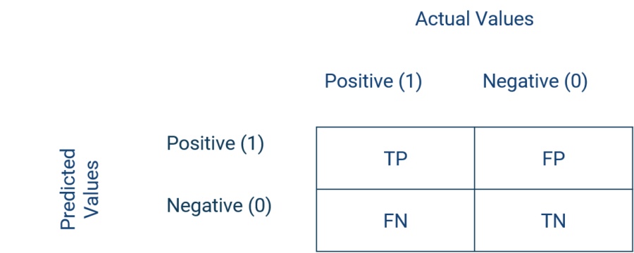
This results in the following performance metrics:
- Accuracy = (TP + TN) / (TP + TN + FP + FN) = (682 + 24) / 760 = 92.9%
- Sensitivity = TP / (TP + FN) = 24 / (24 + 14) = 63.2%
- Specificity = TN / (TN + FP) = 682 / (682 + 40) = 94.5%
- Precision = TP / (TP +FP) = 24 / (24+ 40) = 37.5%
What does the confusion matrix tell me?
The fictitious confusion matrix depicts frequent patterns in reality of unbalanced data sets. If we now consider the accuracy, our model correctly predicts the target variable in about 93% of cases. In absolute terms, this sounds like a very good model. However, let’s consider that the negative class (no purchase) is present in 95% of the cases (722 / 760) and thus, as soon as we would always estimate the negative class, we would correctly predict the target variable in 95% of the cases. This clearly relativizes the predictive power of our model. Of course, in this case the specificity would increase to 100% and the sensitivity would fall to 0%.
How does unbalanced data influence models?
Such models also tend to classify existing observations of the positive (small) class (purchase) as noise and to assign new observations rather to the negative (large) class (no purchase). Our model thus overestimates the negative class (no purchase). However, our model should serve to predict the positive class “purchase ” as correctly as possible.
In our example, it would be disadvantageous not to write potential buyers because they are classified as non-buyers. We assume here that the cost of false negatives is greater than the cost of false positives.
There are three popular methods to reduce or eliminate the class imbalance in the target variable.
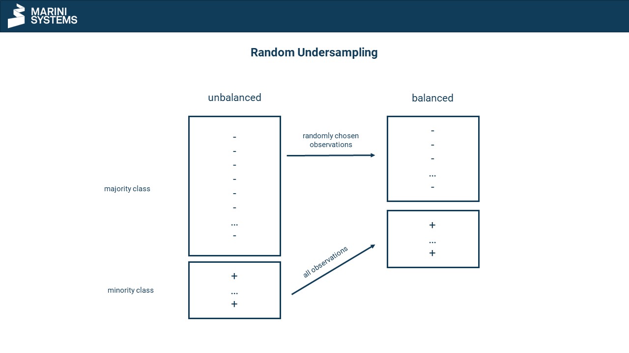
Undersampling
Undersampling involves randomly eliminating observations from the large class from the data set. This results in a more balanced or even balanced data set, depending on the number of eliminated observations. There are also procedures that do not randomly select observations of the large class (condensed nearest neighbours). In doing so, observations that are very similar to others are preferably eliminated. This has the advantage that no observations with high information gain are eliminated.
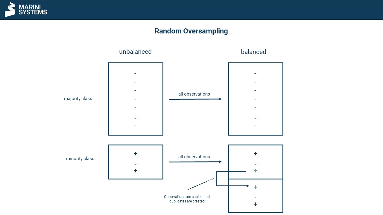
Oversampling
With oversampling, however, the small class is artificially enlarged (see picture below). This is done by randomly copying observations from the small class until the desired balance ratio is reached. However, there is a danger here that models tend overfit afterwards.
A combination of under sampling and oversampling is also possible.
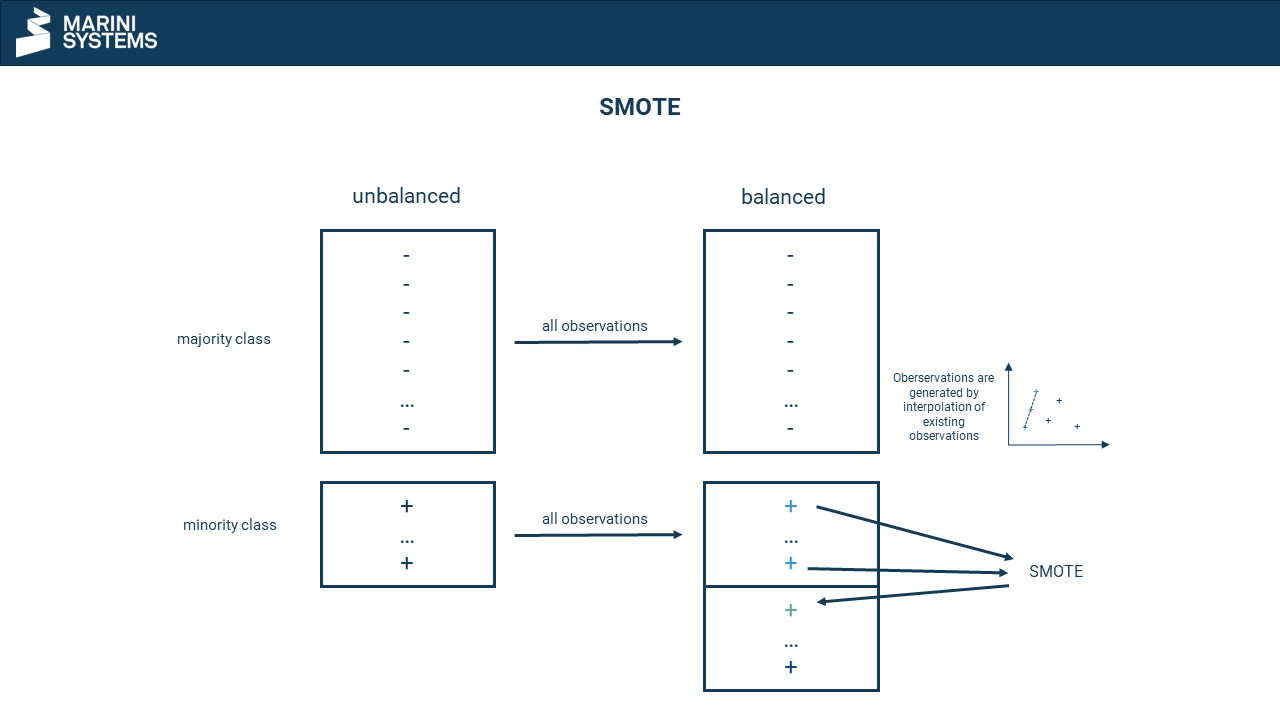
SMOTE
SMOTE stands for Synthetic Minority Oversampling Technique. SMOTE is a method of oversampling. It involves artificially enlarging the small class, but this time not at random. A data point in multivariate space is considered with its k neighbours. Now a vector is taken to one of the neighbours and this vector is multiplied by a random number between 0 and 1. The multiplication is added as a new data point and is now different from the original data point. Thus no copies are made, but new slightly modified data points are synthesized.
Looking for hands-on tutorials in Python to balance your data? We highly recommend the module imbalance-learn!
At Kaggle you also find a very exhaustive tutorial on how to balance your data.
More resources about machine learning
Data integration
How machine learning benefits from data integration
The causal chain “data integration-data quality-model performance” describes the necessity of effective data integration for easier and faster implementable and more successful machine learning. In short, good data integration results in better predictive power of machine learning models due to higher data quality.
From a business perspective, there are both cost-reducing and revenue-increasing effects. The development of the models is cost-reducing (less custom code, thus less maintenance, etc.). Revenue increasing is caused by the better predictive power of the models leading to more precise targeting, cross- and upselling, and more accurate evaluation of leads and opportunities – both B2B and B2C. You can find a detailed article on the topic here:
Platform
How to use machine learning with the Integration Platform
You can make the data from your centralized Marini Integration Platform available to external machine learning services and applications. The integration works seamlessly via the HubEngine or direct access to the platform, depending on the requirements of the third-party provider. For example, one vendor for standard machine learning applications in sales is Omikron. But you can also use standard applications on AWS or in the Google Cloud. Connecting to your own servers is just as easy if you want to program your own models there.
If you need support on how to integrate machine learning models into your platform, please contact our sales team. We will be happy to help you!
Applications
Frequent applications of machine learning in sales
Machine learning can support sales in a variety of ways. For example, it can calculate closing probabilities, estimate cross-selling and up-selling potential, or predict recommendations. The essential point here is that the salesperson is supported and receives further decision-making assistance, which he can use to better concentrate on his actual activity, i.e., selling. For example, the salesperson can more quickly identify which leads, opportunities or customers are most promising at the moment and contact them. However, it remains clear that the salesperson makes the final decision and is ultimately only facilitated by machine learning. In the end, no model sells, but still the human being.
Here you will find a short introduction to machine learning and the most common applications in sales.