Model Evaluation for Machine Learning

The methods random forest, logistic regression and gradient boosting can be categorized in Machine Learning as Supervised Learning. Supervised learning is characterised by the fact that the values of the target variable are known in advance. For example, whether a customer has purchased or not. The values of the target variable are not only needed for model building, but also for model evaluation and selection.

If a data set with n observations is available, it is randomly divided into training and test data sets (e.g. 70/30). The model is “trained” on 70% of the data. The remaining 30% of the data are used to validate the performance of the model. At best, a completely different data set (collected at a different time, in a different place, with other people, etc.) is available. This could be used to determine model performance on independent data, as there is a high probability that the training data and test data are strongly correlated. As a result, model performance tends to be overestimated.

The model selection from several models is based on the model evaluation on the test data set. This contains “unseen” data for the model. Various measures exist for the evaluation of models in case of classification problems. A frequently used measure is derived from the resulting contingency table or confusion matrix. The simplest classification question distinguishes two classes. In the following, the classes describe either a negative (label 0) or positive (label 1) outcome.

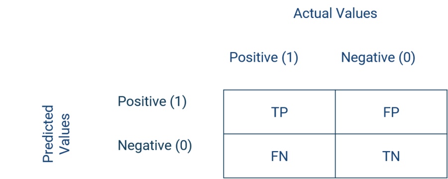
If observations, whose values of the target variable are known, are classified by a model, 4 cells of a contingency table are obtained. The observations that are classified as positive and are positive are called true positives (TP). Likewise, the observations that are classified as negative and are such are called True Negatives (TN). The observations that are classified as negative but are positive are called false negatives (FN). If, on the other hand, the observations are classified as positive but are actually negative, these are called False Positives (FP).

Performance metrics

A metric derived from the contingency table is accuracy (equation 1). It indicates the percentage of observations that were correctly classified. The specificity (equation 2) describes how many percent were correctly classified as positive in relation to all positive observations. Following the same logic, the sensitivity indicates how many percent of all negative observations have been correctly negatively classified, compared to all negative observations.

• Equation 1: Accuracy = (TP+TN) / (TP+FP+TN+FN)
• Equation 2: Specificity = TN / (FP+TN)
• Equation 3: Sensitivity = TP / (FN+TP)

Now models with different model specifications can be trained on the training data and evaluated on the test data based on accuracy, specificity and/or sensitivity (further performance metrics). For example, the model with the highest accuracy can be selected as the final model. This way it is possible to test and evaluate any number of model specifications or algorithms such as random forest or gradient boosting against each other. Of course, this is as usual limited by computational power and time.

The information value is limited if the classes are unequally distributed. For example, if 90% of the observations are positive, an algorithm may tend to classify almost all observations as positive, resulting in a high number of false positives. This results in a high specificity but low sensitivity. In order to take this into account, the so-called Receiver Operating Curve can be determined, whereby 1 minus specificity is plotted on the X-axis and sensitivity on the Y-axis.

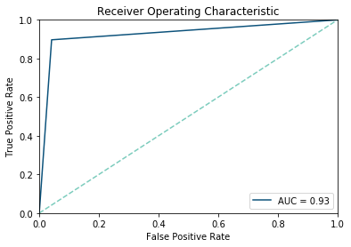
Thus, it represents the relationship between profits (true positives) and costs (false positives). The measure Area Under the Curve (AUC) is derived from this. The AUC value describes the portion under the ROC curve, which can be a maximum of 1 and a minimum of 0. Since Random Guessing classifies correctly in about half of the cases (with a balanced data set), each model should have an AUC value higher than 0.5. Now the AUC value can be used for model selection.

More details can be found here.

Looking for a hands-on tutorial in Python on how to validate your models? Then check out TowardsDataScience!