Decision trees model the relationship between features and a target variable using the structure of a tree. In classification decision trees, the target variable is a categorical (usually binary) variable. The goal is to use the features to predict the membership of a class. By recursive partitioning (dividing the data set) using the features, homogeneous groups are created, which in turn are divided into further homogeneous groups until a stop criterion sets in or the defined homogeneity is reached. The partitioning may be based on various measures such as information gain or the Gini index.
Decision trees start with a root node which contains all observations (top node in the tree shown below). In further steps, the observations are further partitioned by binary splits, e.g. using the Gini index. If a split takes place, all (remaining) features are considered.The one is selected that optimally divides the data into homogeneous groups. Homogeneous means that the group contains a maximum number of observations of one characteristic of the target variable (the more it contains, the purer it is).
Visualized Decision Tree
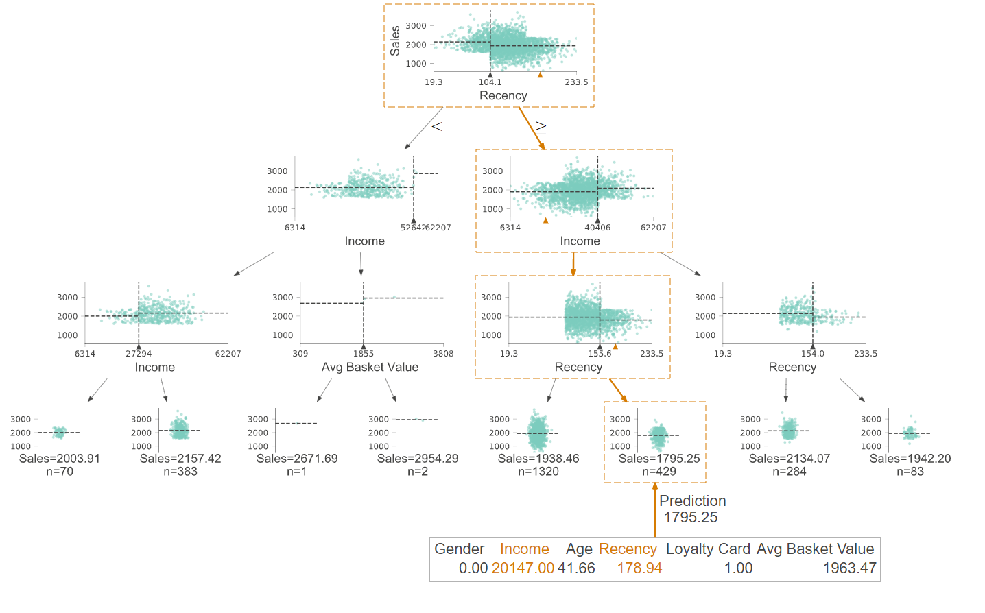
The decision tree above does not represent a categorical target variable, but a continuous one. This means that continuous variables, such as sales, can also be estimated.
Code Snippet
from sklearn.tree import DecisionTreeClassifier
from sklearn.externals.six import StringIO
from IPython.display import Image
from sklearn.tree import export_graphviz
import pydotplus
clf = DecisionTreeClassifier(max_depth=4, criterion = “gini”)
clf = clf.fit(X_train, y_train)
export_graphviz(clf, out_file=dot_data, filled=True, rounded=True, special_characters=True)
graph = pydotplus.graph_from_dot_data(dot_data.getvalue())
Image(graph.create_png())
For more information on coding for Python, see the documentation for scikit-learn.
Explanation of the visualized regression tree
The visualized decision tree represents a regression tree that estimates a continuous target variable. The first split occurs at the root node. If the “recency ” is less than 104.1, the left branch is chosen, otherwise the right branch.
The lowest nodes represent end nodes. The size of the decision tree can be controlled by setting various parameters. In this case the parameters have been set so that no large decision tree is grown (variance bias trade-off). If a new observation (such as the orange path) is to be estimated, the decision tree is run from top to bottom. This shows one strength of decision trees: the ease of interpretation. Furthermore, the variable importance can be inferred. The further top a variable is, the more important it is for the prediction.
Pros and Cons
Pros
- Easy to interpret – thanks to visualization
- Use in many different business contexts
- Specific – serving a specific problem: adding cost or profit functions possible
- White Box Model
Cons
- Instability: Small changes to the data can lead to a completely new tree
- Overfitting: trees can become large and confusing
- Different split criteria result in different trees
More resources about machine learning
Data integration
How machine learning benefits from data integration
The causal chain “data integration-data quality-model performance” describes the necessity of effective data integration for easier and faster implementable and more successful machine learning. In short, good data integration results in better predictive power of machine learning models due to higher data quality.
From a business perspective, there are both cost-reducing and revenue-increasing effects. The development of the models is cost-reducing (less custom code, thus less maintenance, etc.). Revenue increasing is caused by the better predictive power of the models leading to more precise targeting, cross- and upselling, and more accurate evaluation of leads and opportunities – both B2B and B2C. You can find a detailed article on the topic here:
Platform
How to use machine learning with the Integration Platform
You can make the data from your centralized Marini Integration Platform available to external machine learning services and applications. The integration works seamlessly via the HubEngine or direct access to the platform, depending on the requirements of the third-party provider. For example, one vendor for standard machine learning applications in sales is Omikron. But you can also use standard applications on AWS or in the Google Cloud. Connecting to your own servers is just as easy if you want to program your own models there.
If you need support on how to integrate machine learning models into your platform, please contact our sales team. We will be happy to help you!
Applications
Frequent applications of machine learning in sales
Machine learning can support sales in a variety of ways. For example, it can calculate closing probabilities, estimate cross-selling and up-selling potential, or predict recommendations. The essential point here is that the salesperson is supported and receives further decision-making assistance, which he can use to better concentrate on his actual activity, i.e., selling. For example, the salesperson can more quickly identify which leads, opportunities or customers are most promising at the moment and contact them. However, it remains clear that the salesperson makes the final decision and is ultimately only facilitated by machine learning. In the end, no model sells, but still the human being.
Here you will find a short introduction to machine learning and the most common applications in sales.