Cluster Analysis

Cluster analysis belongs to the category of unsupervised learning in machine learning. The aim is to generate k clusters. The clusters should be as heterogeneous among each other as possible and homogeneous within each cluster. Cluster analysis is frequently used, for example, to segment customers and thus to address them more precisely (targeting). The following illustrations are based on real customer data and are intended to illustrate the most important concepts of cluster analysis.

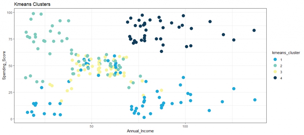
A very popular and established clustering method is the k-Means algorithm. It divides n observations into k-clusters by iteratively minimizing the distances within a cluster and maximizing the distances between the clusters. First, random centroids of k are placed in the multidimensional coordinate system. In a second step, the distances of each observation to each centroid are calculated, then the observations are assigned to the centroid (cluster) to which they are closest. In a third step, the centroids are placed in the center of the cluster. Now steps one to three are repeated until there is no further reassignment of observations to clusters. The number of clusters k and thus the initial centroids must be defined a priori. The figure shows an exemplary visualization of a k-Means method with k = 4 clusters.

This raises the first question: How do you choose the right number of clusters? A possible method for this could be the elbow diagram. It shows the variance against the number of clusters. With the k-Means method, each cluster has a centroid that determines its “center”. Total-Within-Clusters-Sum-Of-Squares (TWSS) is the sum of the squared distances of each observation from its centroid. The smaller the squared sum, the smaller the distance, the higher the similarity. A low TWSS value indicates that the observations are close to their centroids.

In contrast, a high TWSS would indicate that the distances between the observations and their centroids are high, suggesting that the observations are not well distributed to their respective clusters. Finally, the TWSS gives a metric to assess how well the observations are clustered. Since the TWSS decreases with each additional cluster by definition, there is a trade-off between TWSS and the number of clusters. By representing the TWSS and the number of clusters, it is possible to heuristically determine the number of clusters by inference of eye.

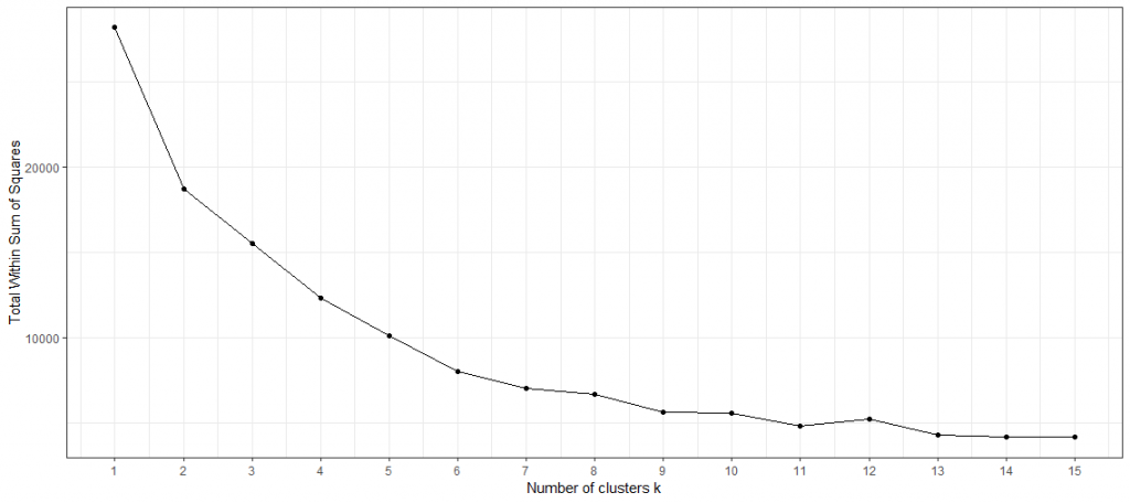
The name is derived from the often seen elbow-like shape of the line chart. The optimal number of clusters based on the elbow chart is not always ambiguous. In general: Choose the k where the line chart has a kink (like an elbow). Here the slope is flattened and thus also the decrease of the TWSS. The elbow diagram above does not show an optimal number of clusters heuristically. Therefore, a different metric must be used for the determination.

If no kink can be seen in the elbow diagram, the silhouette coefficient can be used. It is calculated as follows:

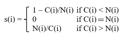
where:

• C(i) = within cluster distance of observation i
• N(i) = closest neighbour distance of observation i

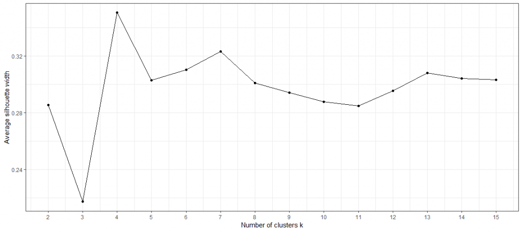
The silhouette coefficient ranges from 1 to -1, where 1 indicates that the observation fits well with its current cluster, 0 indicates that it is at the edge of two clusters and -1 indicates that it fits better with another cluster. After calculating the silhouette coefficient for each individual observation, the average silhouette coefficient can be calculated and used as an overall indicator of how well observations fit into their respective clusters. The higher the average silhouette coefficient, the better each observation fits its cluster on average. On the lower figure of the average silhouette coefficient, the optimal number of clusters is clearly visible with k = 4.

The hierarchical clustering algorithm works differently than the k-Means approach. Though, both use an iterative approach. In the first step of hierarchical clustering, the closest observations (sharing the smallest distance) form a set. In step two, the distance between all other observations and the set from step one is considered. Again, the smallest distance is chosen. If two observations share the smallest distance, they form a new set. If the smallest distance is between an observation and a set, the observation is added to the set. If only sets are left, the distance between the sets is taken into account and the sets are combined. This process is repeated until there is only one final cluster. In this way, a hierarchical structure is created.

Visualization of Hierarchical Clustering

For example, the distance between observations/clusters is determined by the “complete linkage” criterion. In contrast to the k-Means algorithm, the number of clusters is not defined a priori, but posteriorly. By the iterative approach, the result can be visualized in a dendrogram.

You can find a hands-on tutorial in Python in this blog post on TowardsDataScience.